Abstract

• Our method iteratively transports a set of particles to match the target distribution, by applying a form of functional gradient descent that minimizes the KL divergence.
• The derivation of our method is based on a new theoretical result that connects the derivative of KL divergence under smooth transforms with Stein’s identity and a recently proposed kernelized Stein discrepancy.

1. Introduction

target posterior distribution를 구하기 위해서 기존에 세 가지 방법론이 제시되었지만 각각 치명적인 한계를 가지고 있다.

• Bayesian inference : challenge on computing intractable posterior distributions
• Markov chain Monte Carlo (MCMC) : often slow and has difficulty accessing the convergence
• Variational inference : depend on the set of distributions in which the approximation is deinfed

SVGD

• uses a set of particles for approximation. (sampling)
• a form of functional gradient descent is performed to minimize the KL divergence and drive the particles to fit the true posterior distribution.
• simple form.
• can be applied whenever gradient descent can be applied.
• reduces to gradient descent for MAP when using only a single particle (svgd는 bayesian approach의 일반화된 버전이다.)
• based on theoretical result that connects the derivative of KL divergence with respect to smooth variable transforms and kernelized Stein discrepancy

Contents

• Section 2 : Kernelized Stein discrepancy (KSD)
• Section 3 : Connection between KSD and KL divergence
• Section 4 : Related work
• Section 5 : Numerical result
• Section 6 : Conclusion

2. Background

Preliminary

Bayesian inference

• $x$ : continuous random variable or parameter of interest taking values in $\mathcal{X} \subset \mathbf{R}^d$
• $[D_k]$ : a set of independent and identically distributed observation

With $p_0(x)$, Bayesian inference of $x$ involves reasoning with the posterior distribution

Reproducing kernel Hibert space

“함수의 내적으로 임의의 함수를 표현할 수 있다.”

• $k(x, x’) : \mathcal{X} \times \mathcal{X} \rightarrow \mathbf{R}$ : a positive definite kernel

RKHS $\mathcal{H}$ of kernel $k(x, x’)$ : closure of linear span

equipped with inner products

The space of vector-valued function $\mathcal{H}^d (= \mathcal{H} \times \mathcal{H} \times \dots \times \mathcal{H})$ : space of vector functions $\mathbb{f} = [f_1, \dots, f_d]$ with $f_i \in \mathcal{H}$, equipped with inner product

Stein’s Identity and Kernelized Stein Discrepancy

Stein’s identity

• $p(x)$ : continuously differentiable (smooth) density supported on $\mathcal{X} \subseteq \mathbb{R}^d$
• $\mathbf{\phi} (x) = [\phi_1 (x), \phi_2 (x), \dots, \phi_d (x)]^T$ : smooth vector function

For sufficiently regular $\phi$,

where $\mathcal{A}_p = \phi (x) \nabla_x \log p(x)^T + \nabla_x \phi (x)$.

아때 $\mathcal{A}_p$ is Stein operator and $\phi$ is Stein class

Stein discrepancy

• $q(x)$ : smooth density supported in $\mathcal{X}$ different from $p(x)$

The magnitude of $\mathbb{E}_{x \sim q} [ \mathcal{A}_p \phi (x)]$ represent how differnet $p$ and $q$ are. (“maximum violatioin of Stein’s identity”)

For $\phi$ in some proper function set $\mathcal{F}$,

Here the choice of this function set $\mathcal{F}$ is critical, and decides the discriminative power and computational tractability of Stein discrepancy. Traditionally, $\mathcal{F}$ is taken to be sets of functions with bounded Lipschiz norms, which unfortunately casts a challenging functional optimization problem that is computationally intractable or requites special considerations

Kernelized Stein discrepancy

In the unit ball of a Reproducing kernelized Hilbert space로 선정하겠다 그러면 Opt가 closed form solution을 갖는다. 이때 kernel은 stein class여야 한다

3. Variational Inference Using Smooth Transforms

Variational inference approximates the target distribution $p(x)$ using a simpler distribution $q^*(x)$ found in a predefined set $\mathcal{Q} = [q(x)]$ of distributions bu minimizing the KL divergence, that is,

The choice of set $\mathcal{Q}$ is critical and should strike a balance between

1. accuracy : broad enough to closedly approximate a large class of target distributions
2. tractability : consisting of simple distributions that are easy for inference
3. solvability : subsequent KL minimization problem can eb efficiently solved

3.1 Stein Operator as the Derivative of KL Divergence

우리는 variational inference를 tractable하게 하도록 하는 특정한 transformation을 사용할 것이다. 그리고 그 형태는 마치 gradient ascent와 같은 꼴이다.

To explain how we minimize the KL divergence the upper mathematical expression, $\mathbf{T} (x) = x + \epsilon \phi (x)$

• $\phi (x)$ : smooth function that characterizes the perturbation direction
• $\epsilon$ : perturbation magnitude

When $\vert \epsilon \vert$ is sufficiently small, the Jacobian of $T$ is full rank (close to the identitiy matrix), and hence $\mathbf{T}$ is quaranteed to be an one-to-one map by the inverse function theorem.

The following result, which forms the foundation of our method, draws an insightful connection between Stein operator and the derivative of KL divergence w.r.t. the perturbation magnitude $\epsilon$.

Theorem 3.1. Let $\mathbf{T} (x) = x + \epsilon \phi (x)$ and $q_{[\mathbf{T}]} (z)$ the density of $z = \mathbf{T} (x)$ when $x \sim q(x)$,

where $\mathcal{A}_p \phi (x) = \nabla_x \log p(x) \phi (x)^T \nabla_x \phi (x)$ is the Stein operator.

Closed form solution이 사실은 kld를 최소화하는 방향이다.

Lemma 3.2.

Theorem 3.3. Let $\mathbf{T} = x + \mathbb{f} (x), \;\;\; \mathbb{f} \in \mathcal{H}^d$, and $q_{[T]}$ the density of $z = \mathbf{T} (x)$ when $x \sim q$,

whose squared RKHS norm is $\vert\vert \phi_{q, p}^* \vert\vert_{\mathcal{H}^d}^2 = \mathcal{S} (q, p)$.

proof

Thus, Kernelized Stein discrepancy is

for

3.2 Stein Variational Gradient Descent

• 구현할 때 : poster distribution에 대한 expectation을 구할 수 없으니 posterior에서 추출한 샘플에 대한 expectation을 구하자
• Deterministic
• First term and second term

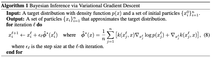
This algorithm mimics a gradient dynamics at the particle level having two terms

• Driving force term : the first term drives the particles towards the high probability areas of $p(x)$ by following a smoothed gradient direction, which is the weighted sum of the gradients of all the points weighted by the kernel function
• Repulsive force term : the second term prevents all the points to collapse together into local modes of $p(x)$

RBF kernel

• If $h \rightarrow 0$, general gradient ascent for maximizing $\log p(x)$.
• If $n = 1$ (single particle), gradient ascent for MAP

Complexity and Efficient Implementation

The major computation bottleneck in (8) lies on calculating $\nabla_x \log p(x)$ for all the points $[x_i]_{i=1}^n$.

We can conveniently address this problem by approximating $\nabla_x \log p(x)$ with subsampled mini-batches $\Omega \subset [1, 2, \dots, N]$ of big data

Additional speedup can be obtained by parallelizing the gradient evaluation of the $n$ particles.

The update (8) requires to compute the kernel matrix $k(x_i, x_j)$ which costs $\mathcal{O} (n^2)$. in paractice this cost can be relatively small compared with the cost of gradient evaluation, since it can be sufficient to use a relatively small $n$ (e.g., several hundreds). If there is a need for very large $n$, one can approximate the summation $\sum_{i=1}$^n by subsampling the particles, or using a random feature expansion of the kernel $k(x, x’)$.

5. Experiments

Radial Basis Function (RBF): RBF 커널은 두 점 간의 거리를 기반으로 작동하여, 데이터 포인트 간의 비선형 관계를 모델링하는 데 도움을 준다.

• $x, x_0$: data point
• $\vert\vert x - x_0 \vert\vert_2^2$: euclidean distance
• $h$: bandwidth 파라미터. RBF kernel의 형태를 결정한다. 대역폭이 크면 더 많은 데이터 포인트가 영향을 미치고, 작으면 가까운 데이터 포인트만 영향을 미친다.
• AdaGrad

Toy Example on 1D Gaussian Mixtur

Target distribution: 두 개의 mode를 갖는 혼합 정규분포

Initial distribution for sampling: target distribution과 충분히 떨어져 있는 분포로 상정한다.

Bayesian Logistic Regression

Bayesian Neural Network

6. Conclusion

We propose a simple purpose variational inference algorithm for fast and scalable Bayesian inference.

Future directions

• more theoretical understanding
• more practical applications in deep learning models
• other potential applications of our basic Theorem in Section 3.

Example of Stein Identity

Stein Identity를 만족하기 위해서는 적절한 smooth vector function $\phi$를 찾는 게 중요하다. 다시 말하면 이는 Stein Identity를 만족하는 $\phi$를 찾는 과정으로도 볼 수 있다.

Gaussian distribution에 대해 Stein Identity를 도출해보자.

Let $R \sim N(\mu, \rho^2), \;\;\; \phi (x) := x - \mu$.

그러면

따라서 Stein Identity가 성립한다.