[Paper Review] NMPC of an Inverted Pendulum
I. Introudction
- Sample interval : 25ms
- Non-convex optimization problem with 61 variables and 241 inequality constraints
II. Nonlinear Model Predictive Control
Discrete-time nonlinear state-space model of dynamic bebaviour
\[x_{k+1} = f_k(x_k, u_k)\]- $x_k \in \mathbb{R}^n$ : state
- $u_k \in \mathbb{R}^m$ : input
- $f_k(., .)$ : function maping the current state and input to the next state
We can predict the state trajectory over a prediction horizon $N$ using the model, so that suitable control action can be taken in order to move the state to the origin.
The state at some point in the future depends only on the initial state $x_1$ and all the inputs from $[u_1, u_2, \cdots, u_N]$.
It is possible to choose an input sequence
that moves the initial state $x_1$ towards a desired region (generally origin).
This goal is achieved by minimizing a cost function
- $Q \in \mathbb{R}^{n \times n}$ : positive semi-definite matrix used to penalise state-movements about the origin
- $R$ : positive definite matrix that penalises input movements from the origin.
NMPC control action is determined by minimising $V_N$ over the future control moves $\mathbf{u}$.
The first control action is applied to the system and the procedure repeats at the next time sample based on new measurements.
Physical limits on the system inputs and states can be directly inclued into the optimization problem.
If the input must line in a set $\mathbb{U}$ and the state must line in a set $\mathbb{X}$ for alll time samples, then the NMPC optimization problem becomes
Solving this problem is non-trivial and usually forms the bulk of the computational work required to obtain the next control action in NMPC. Consquently, the smaple times must be sufficiently large to allow for a solution to be foound.
III. Solving the NMPC Optimization Problem
VI. NMPC Applied to an Inverted Pendulum
- Controlling an inverted pendulum is challenging task becuase it exhibits nonlinear dynamic behaviour, it is unstable about the desired operating point
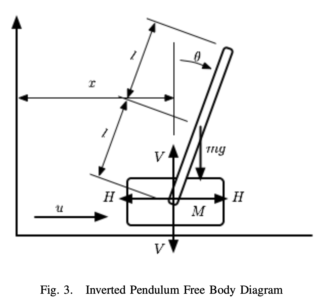
- A cart which can freely move along a straight beam
- Rigid pendulum is attached to the cart and able to rotate freely
- Motor is used to drive the belt, which in turn moves the cart along the rail
- Objective : to swing the pendulum into the upright position and then stabilise the pendulum around this upright position.
- Input : motor (a single input)
- Output : the pendulum angle and the cart position

where $x^T(t) = [p(t), \theta (t), v(t), \omega (t)]$
- $p(t)$ : cart position
- $\theta (t)$ : pendulum angle
- $v(t)$ : cart velocity
- $\omega (t)$ : pendulum angular velocity
The remaining terms
- $\omega_1(x(t), u(t)) = k_1u(t) - (\omega (t))^2 \sin\theta (t) - k_2 u(t)$
- $\omega_2(x(t)) = g\sin\theta (t) - k_3 \omega (t)$
- $d(x(t)) = b - \cos^2\theta (t)$
The constant terms
- $a_1 = \dfrac{J_p}{ml}$
- $a_2 = \dfrac{1}{l}$
- $b = \dfrac{J_p}{ml^2}$
- $k_1 = \dfrac{c_1}{ml}$
- $k_2 = \dfrac{f_c - c_2}{ml}$
- $k_3 = \dfrac{f_p}{ml}$
Where
- $J_p$ : the moment of inertia of the pendulum in relation to the axis or rotation
- $m$ : the equivalent mass of the cart and pendulum
- $l$ : the distance from the axis of ratation to the centre of mass of the system
- $f_c$ : dynamic friction of the cart
- $f_p$ : rotational friction coefficient
- $c_1$ : control force to PWM signal ratio
- $c_2$ : control force to cart velocity ratio